Imputation of phosphoproteomics data with PhosR
8 June 2026
Source:vignettes/web/imputation.Rmd
imputation.RmdIntroduction
PhosR is a package for the all-rounded analysis of
phosphoproteomic data from processing to downstream analysis. This
vignette will provide a step-by-step workflow of how PhosR can be used
to process and analyse a panel of phosphoproteomic datasets. As one of
the first steps of data processing, we will begin by performing
filtering and imputation of the data with PhosR.
Loading packages and data
First, we will load the PhosR package. If you already haven’t done so, please install PhosR as instructed in the main page.
Setting up the data
We assume that you will have the raw data processed using platforms frequently used for mass-spectrometry based proteomics such as MaxQuant. For demonstration purposes, we will take a parts of phosphoproteomic data generated by Humphrey et al. with accession number PXD001792. The dataset contains the phosphoproteomic quantifications of two mouse liver cell lines (Hepa1.6 and FL38B) that were treated with either PBS (mock) or insulin.
Let us load the PhosphoExperiment (ppe) object.
data("phospho.cells.Ins.pe")

ppe <- phospho.cells.Ins.pe
class(ppe)
#> [1] "PhosphoExperiment"
#> attr(,"package")
#> [1] "PhosR"
A quick glance of the object.
ppe
#> class: PhosphoExperiment
#> dim: 5000 24
#> metadata(0):
#> assays(1): Quantification
#> rownames(5000): Q7TPV4;MYBBP1A;S1321;PQSALPKKRARLSLVSRSPSLLQSGVKKRRV
#>   Q3UR85;MYRF;S304;PARAPSPPWPPQGPLSPGTGSLPLSIARAQT ...
#>   P28659-4;NA;S18;AFKLDFLPEMMVDHCSLNSSPVSKKMNGTLD
#>   E9Q8I9;FRY;S1380;HNIELVDSRLLLPGSSPSSPEDEVKDREGEV
#> rowData names(0):
#> colnames(24): Intensity.FL83B_Control_1 Intensity.FL83B_Control_2 ...
#>   Intensity.Hepa1.6_Ins_5 Intensity.Hepa1.6_Ins_6
#> colData names(0):
We will take the grouping information from colnames of
our matrix.
For each cell line, there are two conditions (Control vs Insulin-stimulated) and 6 replicates for each condition.
# FL38B
gsub("Intensity.", "", grps)[1:12]
#>  [1] "FL83B_Control" "FL83B_Control" "FL83B_Control" "FL83B_Control"
#>  [5] "FL83B_Control" "FL83B_Control" "FL83B_Ins"     "FL83B_Ins"
#>  [9] "FL83B_Ins"     "FL83B_Ins"     "FL83B_Ins"     "FL83B_Ins"
# Hepa1
gsub("Intensity.", "", grps)[13:24]
#>  [1] "Hepa1.6_Control" "Hepa1.6_Control" "Hepa1.6_Control" "Hepa1.6_Control"
#>  [5] "Hepa1.6_Control" "Hepa1.6_Control" "Hepa1.6_Ins"     "Hepa1.6_Ins"
#>  [9] "Hepa1.6_Ins"     "Hepa1.6_Ins"     "Hepa1.6_Ins"     "Hepa1.6_Ins"
Note that there are in total 24 samples and 5,000 phosphosites profiled.
dim(ppe)
#> [1] 5000   24
Filtering of phosphosites
Next, we will perform some filtering of phosphosites so that only
phosphosites with quantification for at least 50% of the replicates in
at least one of the conditions are retained. For this filtering step, we
use the selectGrps function. The filtering leaves us with
1,772 phosphosites.
ppe_filtered <- selectGrps(ppe, grps, 0.5, n=1)
dim(ppe_filtered)
#> [1] 1772   24
selectGrps gives you the option to relax the threshold
for filtering. The filtering threshold can therefore be optimized for
each dataset.
# In cases where you have fewer replicates ( e.g.,triplicates), you may want to select phosphosites quantified in 70% of replicates.
ppe_filtered_v1 <- selectGrps(ppe, grps, 0.7, n=1)
dim(ppe_filtered_v1)
#> [1] 1330   24
Imputation of phosphosites
We can proceed to imputation now that we have filtered for suboptimal
phosphosites. To take advantage of data structure and experimental
design, PhosR provides users with a lot of flexibility for imputation.
There are three functions for imputation:
scImpute,tInmpute, and ptImpute.
Here, we will demonstrate the use of scImpute and
ptImpute.
Site- and condition-specific imputation
The scImpute function is used for site- and
condition-specific imputation. A pre-defined thereshold is used to
select phosphosites to impute. Phosphosites with missing values equal to
or greater than a predefined value will be imputed by sampling from the
empirical normal distribution constructed from the quantification values
of phosphosites from the same condition.
In the above example, only phosphosites that are quantified in more than 50% of samples from the same condition will be imputed.
Paired tail-based imputation
We then perform paired tail-based imputation on the dataset imputed
with scImpute. Paired tail-based imputation performs
imputation of phosphosites that have missing values in all
replicates in one condition (e.g. in basal) but not in another
condition (e.g., in stimulation). This method of imputation
ensures that we do not accidentally filter phosphosites that seemingly
have low detection rate.
As for scImpute, we can set a predefined threshold to in
another condition (e.g. stimulation), the tail-based imputation
is applied to impute for the missing values in the first condition.
set.seed(123)
ppe_imputed <- ppe_imputed_tmp
ppe_imputed[,seq(6)] <- ptImpute(ppe_imputed[,seq(7,12)],
                                 ppe_imputed[,seq(6)],
                                 percent1 = 0.6, percent2 = 0, paired = FALSE)
ppe_imputed[,seq(13,18)] <- ptImpute(ppe_imputed[,seq(19,24)],
                                     ppe_imputed[,seq(13,18)],
                                     percent1 = 0.6, percent2 = 0, paired = FALSE)
Lastly, we perform normalisation of the filtered and imputed phosphoproteomic data.
ppe_imputed_scaled <- medianScaling(ppe_imputed, scale = FALSE, assay = "imputed")Quantification plots
A useful function in PhosR is to visualize the
percentage of quantified sites before and after filtering and
imputation. The main inputs of plotQC are the
quantification matrix, sample labels (equating the column names of the
matrix), an integer indicating the panel to plot, and lastly, a color
vector. To visualize the percentage of quantified sites, use the
plotQC function and set panel = quantify to
visualise bar plots of samples.
p1 = plotQC(ppe_filtered@assays@data$Quantification, labels=colnames(ppe_filtered),
        panel = "quantify", grps = grps)
p2 = plotQC(ppe_imputed_scaled@assays@data$scaled,
       labels=colnames(ppe_imputed_scaled), panel = "quantify", grps = grps)
ggpubr::ggarrange(p1, p2, nrow = 1)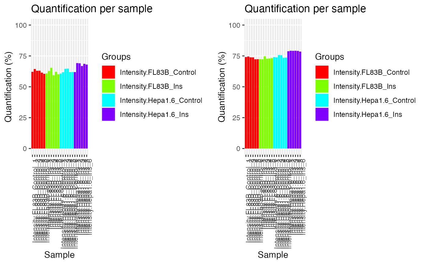
By setting panel = dendrogram, we can visualise the results of unsupervised hierarchical clustering of samples as a dendrogram. The dendrogram demonstrates that imputation has improved the clustering of the samples so that replicates from the same conditions cluster together.
p1 = plotQC(ppe_filtered@assays@data$Quantification,
       labels=colnames(ppe_filtered), panel = "dendrogram",
       grps = grps)
p2 = plotQC(ppe_imputed_scaled@assays@data$scaled,
       labels=colnames(ppe_imputed_scaled),
       panel = "dendrogram", grps = grps)
ggpubr::ggarrange(p1, p2, nrow = 1)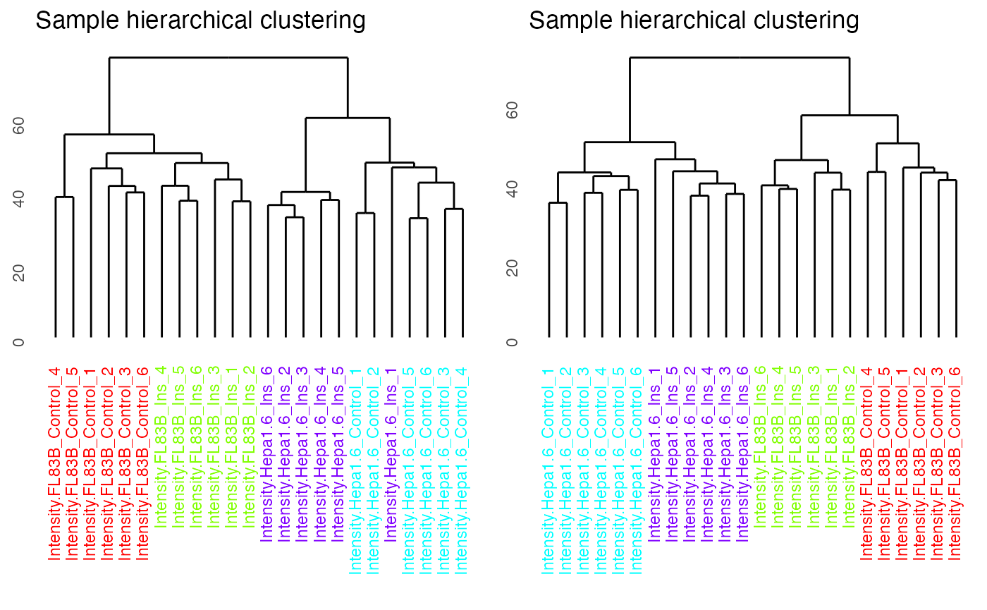
We can now move onto the next step in the PhosR
workflow: integration of datasets and batch correction.
SessionInfo
sessionInfo()
#> R version 4.6.0 (2026-04-24)
#> Platform: x86_64-pc-linux-gnu
#> Running under: Ubuntu 24.04.4 LTS
#>
#> Matrix products: default
#> BLAS:   /usr/lib/x86_64-linux-gnu/openblas-pthread/libblas.so.3
#> LAPACK: /usr/lib/x86_64-linux-gnu/openblas-pthread/libopenblasp-r0.3.26.so;  LAPACK version 3.12.0
#>
#> locale:
#>  [1] LC_CTYPE=C.UTF-8       LC_NUMERIC=C           LC_TIME=C.UTF-8
#>  [4] LC_COLLATE=C.UTF-8     LC_MONETARY=C.UTF-8    LC_MESSAGES=C.UTF-8
#>  [7] LC_PAPER=C.UTF-8       LC_NAME=C              LC_ADDRESS=C
#> [10] LC_TELEPHONE=C         LC_MEASUREMENT=C.UTF-8 LC_IDENTIFICATION=C
#>
#> time zone: UTC
#> tzcode source: system (glibc)
#>
#> attached base packages:
#> [1] stats     graphics  grDevices utils     datasets  methods   base
#>
#> other attached packages:
#> [1] PhosR_1.20.0     BiocStyle_2.40.0
#>
#> loaded via a namespace (and not attached):
#>   [1] gridExtra_2.3               rlang_1.2.0
#>   [3] magrittr_2.0.5              otel_0.2.0
#>   [5] matrixStats_1.5.0           e1071_1.7-17
#>   [7] compiler_4.6.0              systemfonts_1.3.2
#>   [9] vctrs_0.7.3                 reshape2_1.4.5
#>  [11] stringr_1.6.0               pkgconfig_2.0.3
#>  [13] shape_1.4.6.1               fastmap_1.2.0
#>  [15] backports_1.5.1             XVector_0.52.0
#>  [17] labeling_0.4.3              rmarkdown_2.31
#>  [19] markdown_2.0                preprocessCore_1.74.0
#>  [21] ragg_1.5.2                  network_1.20.0
#>  [23] purrr_1.2.2                 xfun_0.58
#>  [25] cachem_1.1.0                litedown_0.9
#>  [27] jsonlite_2.0.0              DelayedArray_0.38.2
#>  [29] broom_1.0.13                R6_2.6.1
#>  [31] bslib_0.11.0                stringi_1.8.7
#>  [33] RColorBrewer_1.1-3          limma_3.68.4
#>  [35] GGally_2.4.0                car_3.1-5
#>  [37] GenomicRanges_1.64.0        jquerylib_0.1.4
#>  [39] Rcpp_1.1.1-1.1              Seqinfo_1.2.0
#>  [41] bookdown_0.46               SummarizedExperiment_1.42.0
#>  [43] knitr_1.51                  IRanges_2.46.0
#>  [45] Matrix_1.7-5                igraph_2.3.2
#>  [47] tidyselect_1.2.1            abind_1.4-8
#>  [49] yaml_2.3.12                 viridis_0.6.5
#>  [51] ggtext_0.1.2                lattice_0.22-9
#>  [53] tibble_3.3.1                plyr_1.8.9
#>  [55] withr_3.0.2                 Biobase_2.72.0
#>  [57] S7_0.2.2                    coda_0.19-4.1
#>  [59] evaluate_1.0.5              desc_1.4.3
#>  [61] ggstats_0.13.0              proxy_0.4-29
#>  [63] xml2_1.5.2                  circlize_0.4.18
#>  [65] pillar_1.11.1               BiocManager_1.30.27
#>  [67] ggpubr_0.6.3                MatrixGenerics_1.24.0
#>  [69] carData_3.0-6               stats4_4.6.0
#>  [71] generics_0.1.4              S4Vectors_0.50.1
#>  [73] ggplot2_4.0.3               commonmark_2.0.0
#>  [75] scales_1.4.0                class_7.3-23
#>  [77] glue_1.8.1                  pheatmap_1.0.13
#>  [79] tools_4.6.0                 dendextend_1.19.1
#>  [81] ggsignif_0.6.4              fs_2.1.0
#>  [83] cowplot_1.2.0               grid_4.6.0
#>  [85] tidyr_1.3.2                 colorspace_2.1-2
#>  [87] Formula_1.2-5               cli_3.6.6
#>  [89] ruv_0.9.7.1                 textshaping_1.0.5
#>  [91] S4Arrays_1.12.0             viridisLite_0.4.3
#>  [93] ggdendro_0.2.0              dplyr_1.2.1
#>  [95] pcaMethods_2.4.0            gtable_0.3.6
#>  [97] rstatix_0.7.3               sass_0.4.10
#>  [99] digest_0.6.39               BiocGenerics_0.58.1
#> [101] SparseArray_1.12.2          htmlwidgets_1.6.4
#> [103] farver_2.1.2                htmltools_0.5.9
#> [105] pkgdown_2.2.0               lifecycle_1.0.5
#> [107] GlobalOptions_0.1.4         statnet.common_4.13.0
#> [109] statmod_1.5.2               gridtext_0.1.6
#> [111] MASS_7.3-65