The `panel` parameter allows different type of visualisation for output object from PhosR. `panel = "all"` is used to create a 2*2 panel of plots including the following. `panel = "quantify"` is used to visualise percentage of quantification after imputataion. `panel = "dendrogram"` is used to visualise dendrogram (hierarchical clustering) of the input matrix. `panel = "abundance"` is used to visualise abundance level of samples from the input matrix. `panel = "pca"` is used to show PCA plot
plotQC(mat, grps, labels, panel =
c("quantify", "dendrogram", "abundance", "pca", "all"))
Arguments
- mat
A p by n matrix, where p is the number of phosphosites and n is the number of samples.
- grps
A vector of colours to be used in the plot. The length should be equal to the columns of the mat.
- labels
A vector of sample names. Used the label points in PCA plot (panel=4)
- panel
A type of plot to output. See description for details.
Value
A graphical plot
Examples
# Imputation
data('phospho.cells.Ins.sample')
grps = gsub('_[0-9]{1}', '', colnames(phospho.cells.Ins))
phospho.cells.Ins.filtered <- selectGrps(phospho.cells.Ins, grps, 0.5, n=1)
set.seed(123)
phospho.cells.Ins.impute <-
scImpute(
phospho.cells.Ins.filtered,
0.5,
grps)[,colnames(phospho.cells.Ins.filtered)]
set.seed(123)
phospho.cells.Ins.impute[,seq_len(5)] <- ptImpute(
phospho.cells.Ins.impute[,seq(6,10)],
phospho.cells.Ins.impute[,seq(5)],
percent1 = 0.6, percent2 = 0, paired = FALSE)
#> idx1: 34
phospho.cells.Ins.ms <- medianScaling(phospho.cells.Ins.impute,
scale = FALSE)
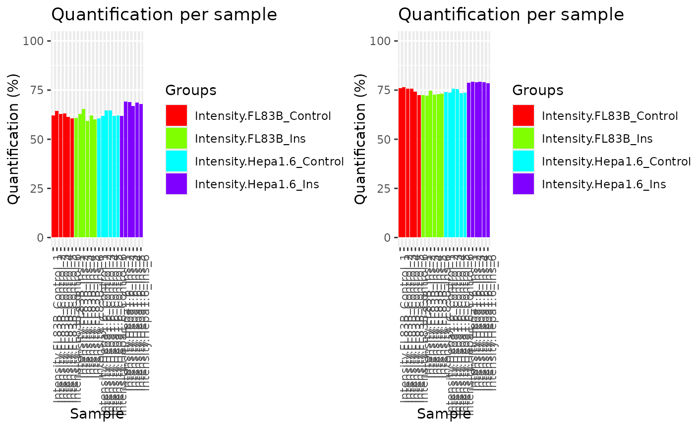
p1 = plotQC(phospho.cells.Ins.filtered,
labels=colnames(phospho.cells.Ins.filtered),
panel = "quantify", grps = grps)
p2 = plotQC(phospho.cells.Ins.ms,
labels=colnames(phospho.cells.Ins.ms),
panel = "quantify", grps = grps)
ggpubr::ggarrange(p1, p2, nrow = 1)
 # Batch correction
data('phospho_L6_ratio_pe')
data('SPSs')
grps = gsub('_.+', '', rownames(
SummarizedExperiment::colData(phospho.L6.ratio.pe))
)
# Cleaning phosphosite label
L6.sites = paste(sapply(GeneSymbol(phospho.L6.ratio.pe),function(x)paste(x)),
";",
sapply(Residue(phospho.L6.ratio.pe), function(x)paste(x)),
sapply(Site(phospho.L6.ratio.pe), function(x)paste(x)),
";", sep = "")
phospho.L6.ratio = t(sapply(split(data.frame(
SummarizedExperiment::assay(phospho.L6.ratio.pe, "Quantification")),
L6.sites),colMeans))
phospho.site.names = split(
rownames(
SummarizedExperiment::assay(phospho.L6.ratio.pe, "Quantification")
), L6.sites)
# Construct a design matrix by condition
design = model.matrix(~ grps - 1)
# phosphoproteomics data normalisation using RUV
ctl = which(rownames(phospho.L6.ratio) %in% SPSs)
phospho.L6.ratio.RUV = RUVphospho(phospho.L6.ratio, M = design, k = 3,
ctl = ctl)
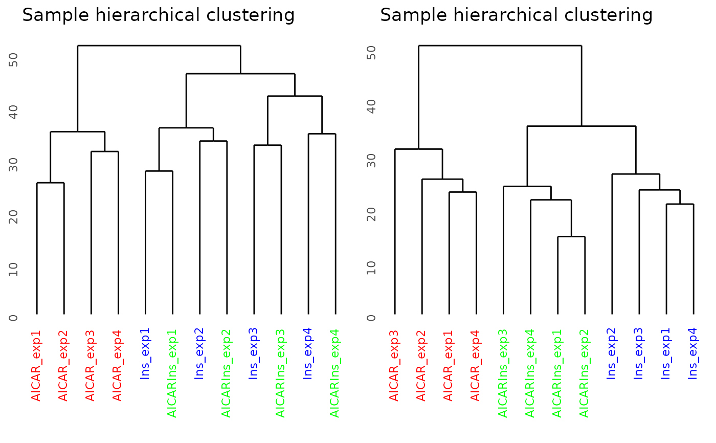
# plot after batch correction
p1 = plotQC(phospho.L6.ratio, panel = "dendrogram", grps=grps,
labels = colnames(phospho.L6.ratio))
p2 = plotQC(phospho.L6.ratio.RUV, grps=grps,
labels = colnames(phospho.L6.ratio),
panel="dendrogram")
ggpubr::ggarrange(p1, p2, nrow = 1)
# Batch correction
data('phospho_L6_ratio_pe')
data('SPSs')
grps = gsub('_.+', '', rownames(
SummarizedExperiment::colData(phospho.L6.ratio.pe))
)
# Cleaning phosphosite label
L6.sites = paste(sapply(GeneSymbol(phospho.L6.ratio.pe),function(x)paste(x)),
";",
sapply(Residue(phospho.L6.ratio.pe), function(x)paste(x)),
sapply(Site(phospho.L6.ratio.pe), function(x)paste(x)),
";", sep = "")
phospho.L6.ratio = t(sapply(split(data.frame(
SummarizedExperiment::assay(phospho.L6.ratio.pe, "Quantification")),
L6.sites),colMeans))
phospho.site.names = split(
rownames(
SummarizedExperiment::assay(phospho.L6.ratio.pe, "Quantification")
), L6.sites)
# Construct a design matrix by condition
design = model.matrix(~ grps - 1)
# phosphoproteomics data normalisation using RUV
ctl = which(rownames(phospho.L6.ratio) %in% SPSs)
phospho.L6.ratio.RUV = RUVphospho(phospho.L6.ratio, M = design, k = 3,
ctl = ctl)
# plot after batch correction
p1 = plotQC(phospho.L6.ratio, panel = "dendrogram", grps=grps,
labels = colnames(phospho.L6.ratio))
p2 = plotQC(phospho.L6.ratio.RUV, grps=grps,
labels = colnames(phospho.L6.ratio),
panel="dendrogram")
ggpubr::ggarrange(p1, p2, nrow = 1)
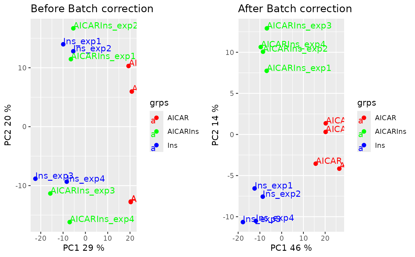
 p1 = plotQC(phospho.L6.ratio, panel = "pca", grps=grps,
labels = colnames(phospho.L6.ratio)) +
ggplot2::ggtitle('Before Batch correction')
p2 = plotQC(phospho.L6.ratio.RUV, grps=grps,
labels = colnames(phospho.L6.ratio),
panel="pca") +
ggplot2::ggtitle('After Batch correction')
ggpubr::ggarrange(p1, p2, nrow = 1)
p1 = plotQC(phospho.L6.ratio, panel = "pca", grps=grps,
labels = colnames(phospho.L6.ratio)) +
ggplot2::ggtitle('Before Batch correction')
p2 = plotQC(phospho.L6.ratio.RUV, grps=grps,
labels = colnames(phospho.L6.ratio),
panel="pca") +
ggplot2::ggtitle('After Batch correction')
ggpubr::ggarrange(p1, p2, nrow = 1)