Batch correction of phosphoproteomics dataset with PhosR
8 June 2026
Source:vignettes/web/batch_correction.Rmd
batch_correction.RmdIntroduction
A common but largely unaddressed challenge in phosphoproteomic data
analysis is to correct for batch effect. Without correcting for batch
effect, it is often not possible to analyze datasets in an integrative
manner. To perform data integration and batch effect correction, we
identified a set of stably phosphorylated sites (SPSs) across a panel of
phosphoproteomic datasets and, using these SPSs, implemented a wrapper
function of RUV-III from the ruv package called
RUVphospho.
Note that when the input data contains missing values, imputation should be performed before batch correction since RUV-III requires a complete data matrix. The imputed values are removed by default after normalisation but can be retained for downstream analysis if the users wish to use the imputed matrix. This vignette will provide an example of how PhosR can be used for batch correction.
Loading packages and data
If you haven’t already done so, load the PhosR package.
In this example, we will use L6 myotube phosphoproteome dataset (with
accession number PXD019127) and the SPSs we identified from a panel of
phosphoproteomic datasets (please refer to the PhosR Cell Reports
paper for the full list of the datasets used). The SPSs
will be used as our negative control in RUV
normalisation.
data("phospho_L6_ratio_pe")
data("SPSs")

ppe <- phospho.L6.ratio.pe
ppe
#> class: PhosphoExperiment
#> dim: 6654 12
#> metadata(0):
#> assays(1): Quantification
#> rownames(6654): D3ZNS8;AAAS;S495;THIPLYFVNAQFPRFSPVLGRAQEPPAGGGG
#>   Q9R0Z7;AAGAB;S210;RSVGSAESCQCEQEPSPTAERTESLPGHRSG ...
#>   D3ZG78;ZZEF1;S1516;SGPSAAEVSTAEEPSSPSTPTRRPPFTRGRL
#>   D3ZG78;ZZEF1;S1535;PTRRPPFTRGRLRLLSFRSMEETRPVPTVKE
#> rowData names(0):
#> colnames(12): AICAR_exp1 AICAR_exp2 ... AICARIns_exp3 AICARIns_exp4
#> colData names(0):
Setting up the data
The L6 myotube data contains phosphoproteomic samples from three treatment conditions each with quadruplicates. Myotube cells were treated with either AICAR or Insulin (Ins), which are both important modulators of the insulin signalling pathway, or both (AICARIns) before phosphoproteomic analysis.
colnames(ppe)[grepl("AICAR_", colnames(ppe))]
#> [1] "AICAR_exp1" "AICAR_exp2" "AICAR_exp3" "AICAR_exp4"
colnames(ppe)[grepl("^Ins_", colnames(ppe))]
#> [1] "Ins_exp1" "Ins_exp2" "Ins_exp3" "Ins_exp4"
colnames(ppe)[grepl("AICARIns_", colnames(ppe))]
#> [1] "AICARIns_exp1" "AICARIns_exp2" "AICARIns_exp3" "AICARIns_exp4"
Note that we have in total 6654 quantified phosphosites and 12 samples in total.
dim(ppe)
#> [1] 6654   12
We have already performed the relevant processing steps to generate a
dense matrix. Please refer to the imputation page to
perform filtering and imputation of phosphosites in order to generate a
matrix without any missing values.
We will extract phosphosite labels.
sites = paste(sapply(ppe@GeneSymbol, function(x)x),";",
                 sapply(ppe@Residue, function(x)x),
                 sapply(ppe@Site, function(x)x),
                 ";", sep = "")
Lastly, we will take the grouping information from
colnames of our matrix.
Diagnosing batch effect
There are a number of ways to diagnose batch effect. In
PhosR, we make use of two visualisation methods to detect
batch effect: dendrogram of hierarchical clustering and a principal
component analysis (PCA) plot. We use the plotQC function
we introduced in the imputation section of the vignette.
By setting panel = dendrogram, we can plot the dendrogram illustrating the results of unsupervised hierarchical clustering of our 12 samples. Clustering results of the samples demonstrate that there is a strong batch effect (where batch denoted as expX, where X refers to the batch number). This is particularly evident for samples from Ins and AICARIns treated conditions.
plotQC(ppe@assays@data$Quantification, panel = "dendrogram", grps=grps, labels = colnames(ppe)) +
  ggplot2::ggtitle("Before batch correction")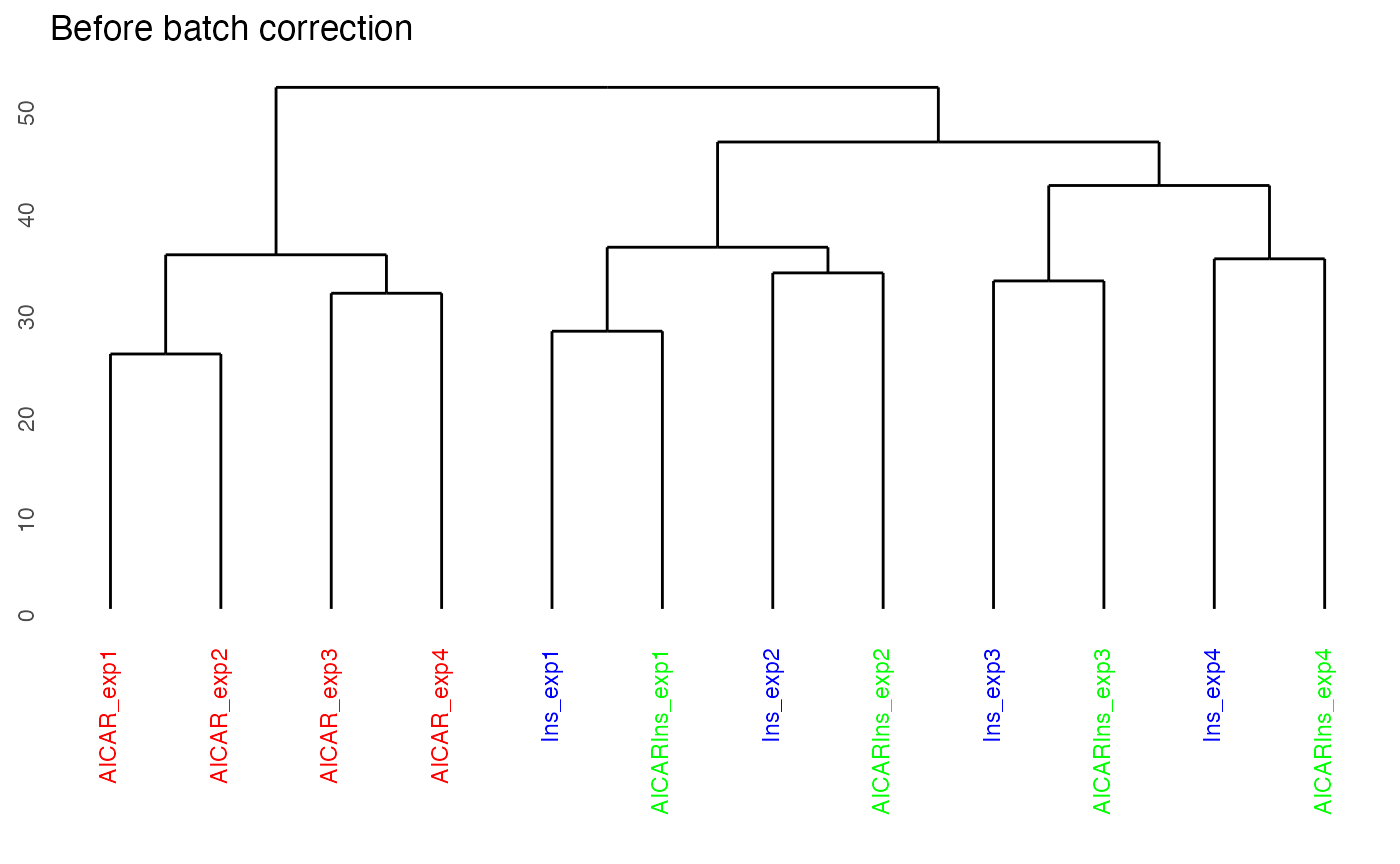
We can also visualise the samples in PCA space by setting panel = pca. The PCA plot demonstrates aggregation of samples by batch rather than treatment groups (each point represents a sample coloured by treatment condition). It has become clearer that even within the AICAR treated samples, there is some degree of batch effect as data points are separated between samples from batches 1 and 2 and those from batches 3 and 4.
plotQC(ppe@assays@data$Quantification, grps=grps, labels = colnames(ppe), panel = "pca") +
  ggplot2::ggtitle("Before batch correction")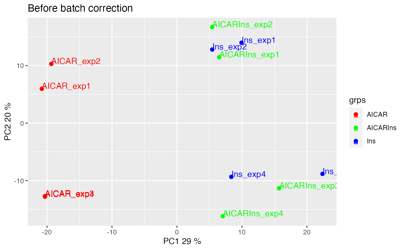
Correcting batch effect
We have now diagnosed that our dataset exhibits batch effect that is
driven by experiment runs for samples treated with three different
conditions. To address this batch effect, we correct for this unwanted
variation in the data by utilising our pre-defined SPSs as a negative
control for RUVphospho.
First, we construct a design matrix by condition.
design = model.matrix(~ grps - 1)
design
#>    grpsAICAR grpsAICARIns grpsIns
#> 1          1            0       0
#> 2          1            0       0
#> 3          1            0       0
#> 4          1            0       0
#> 5          0            0       1
#> 6          0            0       1
#> 7          0            0       1
#> 8          0            0       1
#> 9          0            1       0
#> 10         0            1       0
#> 11         0            1       0
#> 12         0            1       0
#> attr(,"assign")
#> [1] 1 1 1
#> attr(,"contrasts")
#> attr(,"contrasts")$grps
#> [1] "contr.treatment"
We will then use the RUVphospho function to normalise
the data. Besides the quantification matrix and the design matrix, there
are two other important inputs to RUVphospho: 1) the
ctl argument is an integer vector denoting the position of SPSs
within the quantification matrix 2) k parameter is an integer
denoting the expected number of experimental (e.g., treatment)
groups within the data
# phosphoproteomics data normalisation and batch correction using RUV
ctl = which(sites %in% SPSs)
ppe = RUVphospho(ppe, M = design, k = 3, ctl = ctl)
Quality control
As quality control, we will demonstrate and evaluate our
normalisation method with hierarchical clustering and PCA plot using
again plotQC. Both the hierarchical clustering and PCA
results demonstrate the normalisation procedure in PhosR
facilitates effective batch correction.
# plot after batch correction
p1 = plotQC(ppe@assays@data$Quantification, grps=grps, labels = colnames(ppe), panel = "dendrogram" )
p2 = plotQC(ppe@assays@data$normalised, grps=grps, labels = colnames(ppe), panel="dendrogram")
ggpubr::ggarrange(p1, p2, nrow = 1)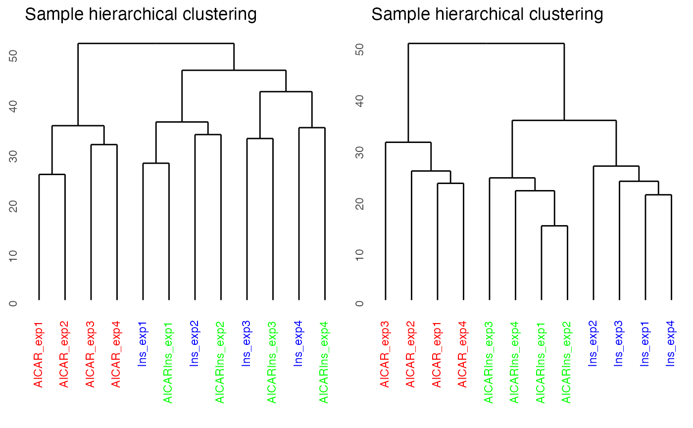
p1 = plotQC(ppe@assays@data$Quantification, panel = "pca", grps=grps, labels = colnames(ppe)) +
  ggplot2::ggtitle("Before Batch correction")
p2 = plotQC(ppe@assays@data$normalised, grps=grps, labels = colnames(ppe), panel="pca") +
  ggplot2::ggtitle("After Batch correction")
ggpubr::ggarrange(p1, p2, nrow = 2)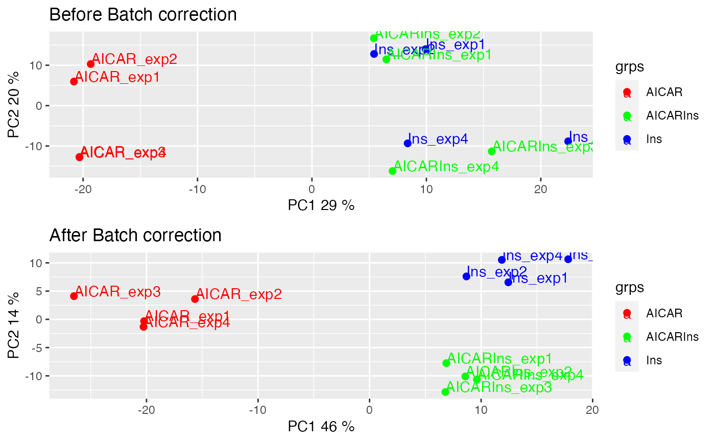
Generating SPSs
We note that the current SPS are derived from
phosphoproteomic datasets derived from mouse cells. To enable users
working on phosphoproteomic datasets derived from other species, we have
developed a function getSPS that takes in multiple
phosphoproteomics datasets stored as phosphoExperiment objects to
generate set of SPS. Users can use their in-house or public
datasets derived from the same speciies to generate species-specific
SPS, which they can use to normalise their data.Below
demonstrate the usage of the getSPS function.
First, load datasets to use for SPS generation.
data("phospho_L6_ratio_pe")
data("phospho.liver.Ins.TC.ratio.RUV.pe")
data("phospho.cells.Ins.pe")

ppe1 <- phospho.L6.ratio.pe
ppe2 <- phospho.liver.Ins.TC.ratio.RUV.pe
ppe3 <- phospho.cells.Ins.pe
Filter, impute, and transform ppe3 (other inputs have already been processed).
grp3 = gsub('_[0-9]{1}', '', colnames(ppe3))
ppe3 <- selectGrps(ppe3, grps = grp3, 0.5, n=1)
ppe3 <- tImpute(ppe3)
FL83B.ratio <- ppe3@assays@data$imputed[, 1:12] - rowMeans(ppe3@assays@data$imputed[,grep("FL83B_Control", colnames(ppe3))])
Hepa.ratio <- ppe3@assays@data$imputed[, 13:24] - rowMeans(ppe3@assays@data$imputed[,grep("Hepa1.6_Control", colnames(ppe3))])
ppe3@assays@data$Quantification <- cbind(FL83B.ratio, Hepa.ratio)
Generate inputs of getSPS.
ppe.list <- list(ppe1, ppe2, ppe3)
cond.list <- list(grp1 = gsub("_.+", "", colnames(ppe1)),
                  grp2 = str_sub(colnames(ppe2), end=-5),
                  grp3 = str_sub(colnames(ppe3), end=-3))
Finally run getSPS to generate list of SPSs.
inhouse_SPSs <- getSPS(ppe.list, conds = cond.list)

head(inhouse_SPSs)
#> [1] "TMPO;S67;"    "RBM5;S621;"   "SRRM1;S427;"  "THOC2;S1417;" "SSB;S92;"
#> [6] "PPIG;S252;"
Run RUVphospho using the newly generateed SPSs.
(NOTE that we do not expect the results to be
reproducible as the exempler SPSs have been generated from dummy
datasets that have been heavily filtered.)
SessionInfo
sessionInfo()
#> R version 4.6.0 (2026-04-24)
#> Platform: x86_64-pc-linux-gnu
#> Running under: Ubuntu 24.04.4 LTS
#>
#> Matrix products: default
#> BLAS:   /usr/lib/x86_64-linux-gnu/openblas-pthread/libblas.so.3
#> LAPACK: /usr/lib/x86_64-linux-gnu/openblas-pthread/libopenblasp-r0.3.26.so;  LAPACK version 3.12.0
#>
#> locale:
#>  [1] LC_CTYPE=C.UTF-8       LC_NUMERIC=C           LC_TIME=C.UTF-8
#>  [4] LC_COLLATE=C.UTF-8     LC_MONETARY=C.UTF-8    LC_MESSAGES=C.UTF-8
#>  [7] LC_PAPER=C.UTF-8       LC_NAME=C              LC_ADDRESS=C
#> [10] LC_TELEPHONE=C         LC_MEASUREMENT=C.UTF-8 LC_IDENTIFICATION=C
#>
#> time zone: UTC
#> tzcode source: system (glibc)
#>
#> attached base packages:
#> [1] stats     graphics  grDevices utils     datasets  methods   base
#>
#> other attached packages:
#> [1] stringr_1.6.0 PhosR_1.20.0
#>
#> loaded via a namespace (and not attached):
#>   [1] gridExtra_2.3               rlang_1.2.0
#>   [3] magrittr_2.0.5              otel_0.2.0
#>   [5] matrixStats_1.5.0           e1071_1.7-17
#>   [7] compiler_4.6.0              systemfonts_1.3.2
#>   [9] vctrs_0.7.3                 reshape2_1.4.5
#>  [11] pkgconfig_2.0.3             shape_1.4.6.1
#>  [13] fastmap_1.2.0               backports_1.5.1
#>  [15] XVector_0.52.0              labeling_0.4.3
#>  [17] rmarkdown_2.31              markdown_2.0
#>  [19] preprocessCore_1.74.0       ragg_1.5.2
#>  [21] network_1.20.0              purrr_1.2.2
#>  [23] xfun_0.58                   cachem_1.1.0
#>  [25] litedown_0.9                jsonlite_2.0.0
#>  [27] DelayedArray_0.38.2         broom_1.0.13
#>  [29] R6_2.6.1                    bslib_0.11.0
#>  [31] stringi_1.8.7               RColorBrewer_1.1-3
#>  [33] limma_3.68.4                GGally_2.4.0
#>  [35] car_3.1-5                   GenomicRanges_1.64.0
#>  [37] jquerylib_0.1.4             Rcpp_1.1.1-1.1
#>  [39] Seqinfo_1.2.0               SummarizedExperiment_1.42.0
#>  [41] knitr_1.51                  IRanges_2.46.0
#>  [43] Matrix_1.7-5                igraph_2.3.2
#>  [45] tidyselect_1.2.1            abind_1.4-8
#>  [47] yaml_2.3.12                 viridis_0.6.5
#>  [49] ggtext_0.1.2                lattice_0.22-9
#>  [51] tibble_3.3.1                plyr_1.8.9
#>  [53] withr_3.0.2                 Biobase_2.72.0
#>  [55] S7_0.2.2                    coda_0.19-4.1
#>  [57] evaluate_1.0.5              desc_1.4.3
#>  [59] ggstats_0.13.0              proxy_0.4-29
#>  [61] xml2_1.5.2                  circlize_0.4.18
#>  [63] pillar_1.11.1               BiocManager_1.30.27
#>  [65] ggpubr_0.6.3                MatrixGenerics_1.24.0
#>  [67] carData_3.0-6               stats4_4.6.0
#>  [69] generics_0.1.4              S4Vectors_0.50.1
#>  [71] ggplot2_4.0.3               commonmark_2.0.0
#>  [73] scales_1.4.0                BiocStyle_2.40.0
#>  [75] class_7.3-23                glue_1.8.1
#>  [77] pheatmap_1.0.13             tools_4.6.0
#>  [79] dendextend_1.19.1           ggsignif_0.6.4
#>  [81] fs_2.1.0                    cowplot_1.2.0
#>  [83] grid_4.6.0                  tidyr_1.3.2
#>  [85] colorspace_2.1-2            Formula_1.2-5
#>  [87] cli_3.6.6                   ruv_0.9.7.1
#>  [89] textshaping_1.0.5           S4Arrays_1.12.0
#>  [91] viridisLite_0.4.3           ggdendro_0.2.0
#>  [93] dplyr_1.2.1                 pcaMethods_2.4.0
#>  [95] gtable_0.3.6                rstatix_0.7.3
#>  [97] sass_0.4.10                 digest_0.6.39
#>  [99] BiocGenerics_0.58.1         SparseArray_1.12.2
#> [101] htmlwidgets_1.6.4           farver_2.1.2
#> [103] htmltools_0.5.9             pkgdown_2.2.0
#> [105] lifecycle_1.0.5             GlobalOptions_0.1.4
#> [107] statnet.common_4.13.0       statmod_1.5.2
#> [109] gridtext_0.1.6              MASS_7.3-65