Cell-level representation learning¶

The goal: turn raw, multi-batch, multi-modal single-cell data into one clean embedding, a handful of coordinates per cell that mix the batches together while keeping the biology, so you can cluster and analyze all your data as one.

This runs on the built-in Liu et al. COVID-19 subsample (~30k cells, 3 batches, RNA + ADT).

library(m3)
set.seed(0)

1. Load the demo dataset¶

m3_demo() returns a ready-to-use m3_dataset, a subsample of the Liu et al. COVID-19 CITE-seq data (RNA + ADT), with the obs columns already set up.

data <- m3_demo()
data
#> m3_dataset(n_cells=30534, batches=[B1, B2, B3], modalities=[rna:1000, adt:192])

2. Build and train the model¶

m3_train(...) sets up the model from your data and fits it, telling it which obs columns to use:

condition_keys, the conditions you're comparing across (here disease group + age band).
celltype_key, the column holding cell-type labels.
batch_key, the column marking which batch each cell is from (B1/B2/B3). The model corrects for batch, so cells group by biology rather than by batch.
embedding_dim, how many numbers describe each cell in the output (here 30).

donor_prediction = FALSE fits only the integration model and skips the disease-prediction step (not needed for embeddings, and faster). seed = 0 makes the run reproducible. Afterwards m3_capabilities(model) shows which outputs are available.

#To save time, users can set max_epochs to 100 for test.
model <- m3_train(
  data,
  condition_keys = c("cond_group", "Age_interval"),
  celltype_key   = "mergedcelltype",
  batch_key      = "batch",
  embedding_dim  = 30L,
  donor_prediction = FALSE,
  max_epochs = 500L,
  seed = 0L
)
#> Using 'matrix/data'
#> torch.Size([1000, 7163])
#> Using 'matrix/data'
#> torch.Size([1000, 10789])
#> Using 'matrix/data'
#> torch.Size([1000, 12582])
#> Using 'matrix/data'
#> torch.Size([192, 7163])
#> Using 'matrix/data'
#> torch.Size([192, 10789])
#> Using 'matrix/data'
#> torch.Size([192, 12582])
#> Batch counts: {0: 7163, 1: 10789, 2: 12582}
#> Minimum batch size: 7163
#> Epoch 1, Validation Loss: 5.1807
#> Epoch 2, Validation Loss: 5.1167
#> Epoch 3, Validation Loss: 5.0486
#> ...  (494 epochs omitted)  ...
#> Epoch 498, Validation Loss: 0.5032
#> Epoch 499, Validation Loss: 0.5039
#> Epoch 500, Validation Loss: 0.5011
#> Using 'matrix/data'
#> torch.Size([1000, 7163])
#> Using 'matrix/data'
#> torch.Size([1000, 10789])
#> Using 'matrix/data'
#> torch.Size([1000, 12582])
#> Using 'matrix/data'
#> torch.Size([192, 7163])
#> Using 'matrix/data'
#> torch.Size([192, 10789])
#> Using 'matrix/data'
#> torch.Size([192, 12582])
model
#> m3_model
#>   modalities     : rna, adt (embedding_dim=30)
#>   condition keys : cond_group, Age_interval  (target: cond_group)
#>   roles          : celltype=mergedcelltype  donor=-  batch=batch
#>   capabilities   : embedding, reconstruct
m3_capabilities(model)
#>      embedding    reconstruct predict_donors 
#>           TRUE           TRUE          FALSE

3. Get the embedding¶

m3_embedding(model, part = ...) returns the trained coordinates as a cells x embedding_dim matrix. Ask for the part you want by name:

"bio", the biological signal, with batch differences removed. This is the one you cluster and analyze.
"batch", the batch signal on its own, if you ever want to inspect it separately.

m3_cell_metadata(model) is the per-cell obs table, row-aligned with the embedding.

emb_bio       <- m3_embedding(model, part = "bio")
emb_intrinsic <- m3_embedding(model, part = "intrinsic")
emb_batch     <- m3_embedding(model, part = "batch")
meta <- m3_cell_metadata(model)
cat(sprintf("bio: %s | intrinsic: %s | batch: %s\n",
            paste(dim(emb_bio), collapse = "x"),
            paste(dim(emb_intrinsic), collapse = "x"),
            paste(dim(emb_batch), collapse = "x")))
#> bio: 30534x28 | intrinsic: 30534x24 | batch: 30534x2

4. Save the embedding + metadata¶

Save the embedding and its metadata. m3 returns plain matrices, so persist them however you like, here as CSV and an .rds.

out <- file.path(tempdir(), "m3_tut1")
dir.create(out, showWarnings = FALSE)
utils::write.csv(emb_bio, file.path(out, "embedding_bio.csv"), row.names = FALSE)
utils::write.csv(meta, file.path(out, "cell_metadata.csv"), row.names = FALSE)
saveRDS(list(embedding = emb_bio, metadata = meta), file.path(out, "embedding_bio.rds"))
cat("saved embedding to", out, "\n")
#> saved embedding to /tmp/RtmpavmnOE/m3_tut1

5. Visualise with UMAP¶

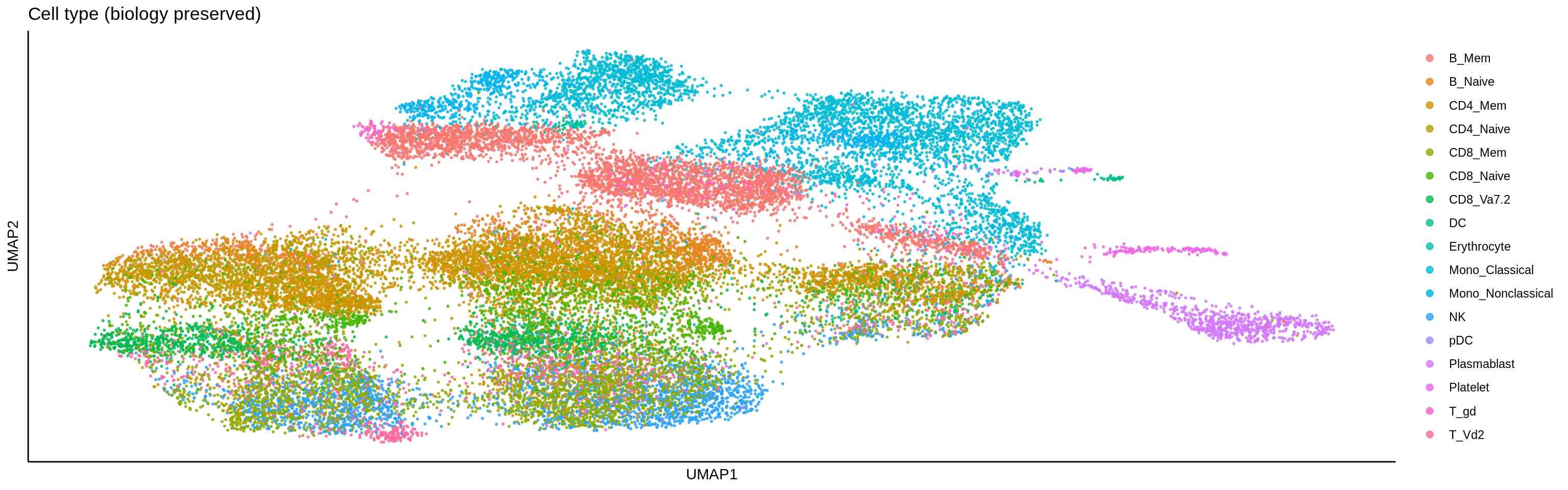
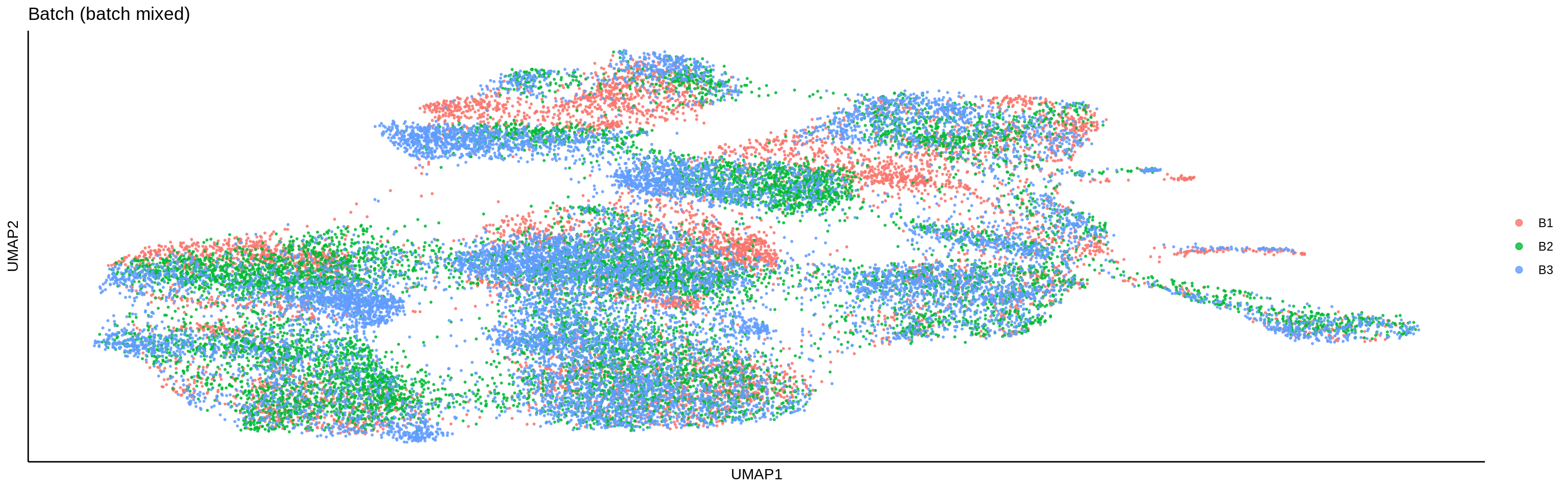
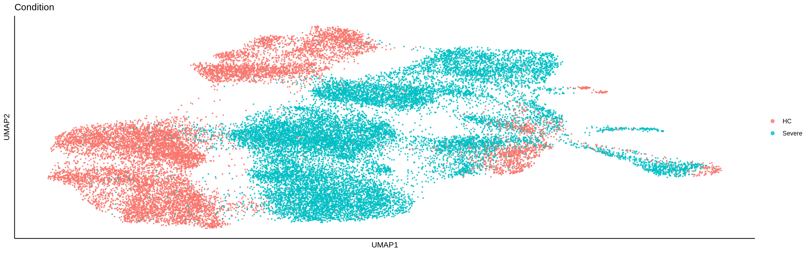
A UMAP of the "bio" embedding. If integration worked, cells should group by cell type (biology kept) while the batches mix together (batch difference removed), colour by each to check.

xy <- m3_umap(emb_bio, method = "scanpy", n_neighbors = 15L, device = model$device)
df <- data.frame(UMAP1 = xy[, 1], UMAP2 = xy[, 2],
                 celltype = factor(meta$mergedcelltype),
                 batch    = factor(meta$batch),
                 condition = factor(meta$cond_group))

plt <- function(colour, title, legend = TRUE) {
  ggplot(df, aes(UMAP1, UMAP2, colour = .data[[colour]])) +
    geom_point(size = 0.4, alpha = 0.8) +
    theme_classic() +
    theme(axis.text = element_blank(), axis.ticks = element_blank(),
          legend.position = if (legend) "right" else "none") +
    guides(colour = guide_legend(override.aes = list(size = 2))) +
    labs(title = title, colour = NULL)
}
print(plt("celltype",  "Cell type (biology preserved)"))

print(plt("batch",     "Batch (batch mixed)"))

print(plt("condition", "Condition"))

Done. You now have an integrated cell embedding, ready for clustering and downstream analysis. The patient-prediction tutorial builds on the same model to predict donor-level disease status.